What are Optimizers and Loss Functions?

Optimizers and loss functions are pivotal elements in the training process of a deep learning model. Loss functions, often referred to as cost functions, play a critical role in evaluating the model’s performance by quantifying the disparity between its predictions and the ground truth or actual values. Conversely, optimizers act as functions that dynamically adjust the model’s weights and parameters towards values that minimize the computed loss. Optimizer and loss functions are complementary functions to each other, which work together to enhance the model’s capabilities through iterative parameter updates during the training phase.

Loss Functions

There are numerous loss function implementations have been provided by deep learning frameworks like PyTorch, TensorFlow etc. which can be used according to the requirements. Some of the widely used loss functions, such as MSE (Mean Squared Error), MAE (Mean Absolute error), BCE (Binary Cross Entropy), CCE (Categorical Cross Entropy) are explained below.

Mean Squared Error (MSE)

Mean Squared Error (MSE) quantifies the average squared difference between the predicted values and the actual target values. The MSE loss function is particularly useful when training neural networks for regression problems, where the goal is to predict continuous values. MSE can be defined using below mathematical formula.

$$MSE=\frac{1}{n}\sum_{i=1}^n(y_{p}-y_{a})^2$$

n is the number of examples in dataset.
y_p is the predicted value of i^th example.
y_a is the actual value of i^th example.

The difference between predicted and actual value is squared because MSE amplifies larger errors, giving more weight to instances where the model’s predictions deviate significantly from the true values.

Mean Absolute Error (MAE)

Mean Absolute Error(MAE) serves as a frequently employed loss function in regression analysis. In contrast to Mean Squared Error (MSE), where the squared differences between predicted and actual values are averaged, MAE calculates the average absolute difference between these values, providing a metric that directly reflects the magnitude of errors without squaring them. MSE can be defined using below mathematical formula.

$$MAE=\frac{1}{n}\sum_{i=1}^n|y_{p}-y_{a}|$$

n is the number of examples in dataset.
y_p is the predicted value of i^th example.
y_a is the actual value of i^th example.

MAE has a linear impact on errors. Large errors contribute proportionally to the overall metric without being squared, providing a more balanced representation of the model’s performance.

Binary Cross Entropy (BCE)

This is a loss function which is mostly used in binary classification models. In other words, it is particularly suitable when the output of the model is a probability score indicating the likelihood of an instance belonging to the positive class (class 1). BCE can be defined using below mathematical formula.

$$BCE=-\frac{1}{n}\sum_{i=1}^n(y_{a}log(y_{p})+(1-y_{a})log(1-y_{p}))$$

n is the number of examples in dataset.
y_p is the predicted value of i^th example.
y_a is the actual value of i^th example.

BCE is relatively simple and computationally efficient. It is specifically designed for binary classification tasks and involves the calculation of the log-likelihood between the true labels and the predicted probabilities for each example.

Categorical Cross Entropy (CCE)

Categorical Cross entropy is a loss function commonly used in machine learning, especially in the context of multiclass classification problems. It measures the dissimilarity between the predicted probability distribution and the true probability distribution of class labels.

In a classification task with C classes, where each example has a true label y_actual (a one-hot encoded vector) and a predicted probability distribution y_predict (output from the model’s softmax function), the Categorical Cross entropy loss is calculated as:

$$CCE=-\frac{1}{n}\sum_{i=1}^n\sum_{j=1}^Cy_{a}log(y_{p})$$

C is the number of classes.
y_a is the true probability distribution for class j of example i.
y_p is the predicted probability distribution for class j of example i.

Categorical Cross Entropy is often used in combination with the softmax activation function in the output layer of a neural network for multiclass classification. The softmax function converts raw model outputs into normalized probabilities.

Sparse Cross Entropy (SCE)

Sparse Cross Entropy is similar to Categorical Cross Entropy (CCE) but used when the class labels are integers.

$$SCE=-\frac{1}{n}\sum_{i=1}^nlog(y_{predict})$$

n is the number of examples in dataset.
y_predict is the predicted probability distribution for example i.

Optimizers

An optimizer is an algorithm or method used to adjust the parameters of a model in order to minimize the error or loss function during training. The goal of optimization is to find the optimal set of parameters that allow the model to make accurate predictions on new, unseen data. During training, the model is presented with a set of input data along with corresponding target labels. The optimizer adjusts the model’s parameters based on the difference between the model’s predictions and the true labels, as quantified by the chosen loss function. One of the widely known optimizing algorithm in machine leaning is Gradient Descent.

Gradient Descent

Gradient Descent is an iterative optimization algorithm used to minimize the cost or loss function in the context of machine learning and optimization problems. The primary goal of Gradient Descent is to find the minimum of a function by iteratively moving in the direction of steepest descent. Here’s a basic overview of how Gradient Descent works.

Given an objective or cost function J(θ), where θ represents the parameters of a model (weights and biases), the goal is to find the values of θ that minimize J(θ).
Initialize the parameters θ with some arbitrary values.
Calculate the gradient of the cost function with respect to each parameter. The gradient is a vector that points in the direction of the steepest increase in the cost function.
Adjust the parameters θ in the opposite direction of the gradient to minimize the cost. The update rule is typically of the form as θ=θ−α∇J(θ). Here, α is the learning rate, a hyperparameter that determines the step size of each iteration.
Repeat steps 3-4 until convergence or a predetermined number of iterations. Convergence is typically determined by monitoring changes in the cost function or the norm of the gradient.

Let’s understand it using gradient descent curve.

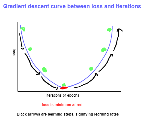
(b. Challenge with higher learning rate)

(c. Challenge with very low learning rate)

The provided images depict Gradient Descent curves with varying learning rates. The process begins by selecting arbitrary values for the weights, which are iteratively adjusted to minimize the loss. In the diagrams, the direction of black arrow indicates the direction of optimization. The loss consistently decreases with each epoch, ultimately reaching the red point, representing the minimum, hence termed Gradient Descent. This represents the ideal state, beyond which the loss begins to increase again. The distance between two green points (black arrow) is referred to as the learning rate, a crucial hyperparameter that must be chosen efficiently to ensure the model achieves minimum loss.

In image (b), it is evident that the chosen learning rate is excessively large, leading to a tendency to bypass the local minimum (red point). Consequently, the model experiences an increase in loss once again.

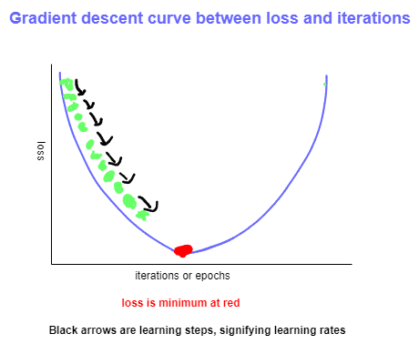
In image (c), it is observed that the chosen learning rate is exceedingly low, causing the model to progress very slowly and making it less likely to reach the minimum. Therefore, opting for an extremely low learning rate is also not advisable.

To attain optimal performance from the model, it is imperative to carefully select the learning rate, ensuring that the model can reach the lowest loss, represented by the red point in image (a).

There are various variants available of Gradient descent, which are explained below.

Gradient Descent with Momentum

Gradient Descent with Momentum is an optimization algorithm that enhances the standard Gradient Descent method by incorporating a momentum term. The momentum helps accelerate the optimization process, particularly in the presence of flat regions, oscillations, and saddle points. Here’s how Gradient Descent with Momentum works.

In standard Gradient Descent, the update rule for adjusting the parameters (θ) is given by θ=θ−α∇J(θ). Here, α is the learning rate, a hyperparameter that determines the step size of each iteration. If the value of gradient of cost function (∇J(θ)) is zero, parameters (θ) are not going to be updated, hence the optimization process with stuck. The point where the derivative is turning to zero, is called Saddle point. Below image is explaining saddle point.

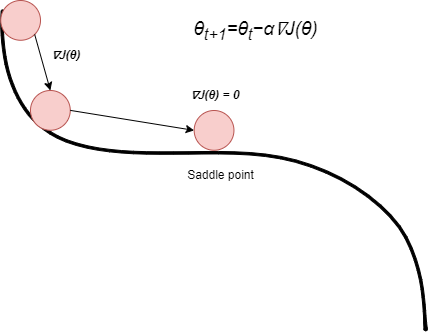
When the derivative of the cost function (∇J(θ)) becomes zero, resulting in θ_t+1 being equal to θ_t. Consequently, the optimization process gets stuck, even if it hasn’t reached a minimum (the point where the loss is minimum). In the picture above, think of a ball stuck on a flat spot, like a saddle point. It won’t roll down to the minimum (the downhill) unless someone gives it a push. This is precisely where the significance of momentum comes into play, preventing such stagnation and allowing the optimization process to efficiently navigate through the parameter space. We calculate the velocity at each iteration by multiplying the previous iteration velocity with momentum and add that to calculated gradient (∇J(θ)). So, even if the gradient is zero at saddle point, the optimization will not be stuck and will reach to the minimum point (point where the loss is minimum).

Explaining with the equations below:

Standard Gradient Descent	θ_t+1=θ_t−α∇J(θ), where α is learning rate and ∇J(θ) is a derivative of cost function.
Gradient Descent with Momentum	θ_t+1=θ_t−αv_t+1, where α is learning rate and v_t+1 is a velocity at t+1. Velocity can be defined as, v_t+1 = ρv_t + ∇J(θ), where ρ is a momentum, v_t is the previous velocity, and ∇J(θ) is a derivative of cost function.

Another problem is Local Minima, where Gradient descent with momentum can help to overcome. Lets consider our ball example to understand local minima.

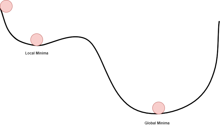
Local Minima

Local Minima is the point, where the loss is minimum within the small neighbourhood, but that is not a global minimum, where we want to reach. At local minimum, the derivative of cost function will be negative, using the ball analogy in above image, it will be forcing the ball to roll in the direction of local minimum. Here, we can apply the momentum, which will force the ball in the opposite direction of the derivative, leading to push it to global minimum. We need to be careful while deciding the momentum value here, extremely low momentum can result in the ball not reaching till global minimum, and extremely large momentum may result in the ball overshooting the global minimum. We need the ball to stop at a global minimum.

There are several other variants of the gradient descent algorithm, each designed to address specific challenges or improve the convergence speed in certain scenarios. Here are some popular variants of gradient descent:

Batch Gradient Descent

Batch Gradient Descent is a traditional gradient descent where the entire dataset is used to compute the gradient of the cost function in each iteration. Batch Gradient Descent is applied at epoch level, or for each iteration.

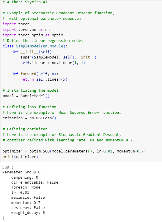
Stochastic Gradient Descent

Instead of using the entire dataset in each iteration, SGD uses only one randomly selected data point to update the parameters. This can lead to faster updates but introduces more variance. Example of SGD with momentum in PyTorch is below:

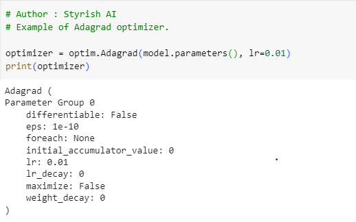
Adagrad (Adaptive Gradient Algorithm)

Adagrad is an optimizer featuring parameter-specific learning rates that dynamically adjust based on how frequently each parameter is updated during training. This adaptive strategy allocates larger learning rates to parameters with less frequent updates and smaller learning rates to frequently updated parameters. However, Adagrad comes with a drawback: the learning rate for each parameter is scaled according to the historical sum of squared gradients. As training progresses, this accumulation of squared gradients can lead to a continuous diminution of the learning rate. Consequently, if the training duration is extended, the persistently decreasing learning rates may impede the optimization process from converging as expected, causing prolonged and unexpected durations to reach the minimum (see image(c) in gradient descent curves). Below is the example of Adagrad:

To overcome the limitation from Adagrad, RMSProp has been introduced.

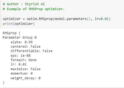
RMSProp (Root Mean Square Propagation)

As previously mentioned, this particular optimization method serves to address the limitations of the Adagrad optimizer. In Adagrad, the squared gradient factor tends to increase continuously for frequently updated parameters due to its accumulation mechanism, leading to a persistent decrease in the learning rate. In contrast, RMSProp operates by employing a moving average of squared gradients instead of accumulating them, effectively averting rapid diminishment of learning rates during training. This approach allows the optimization process to better adapt to the characteristics of the data, promoting more effective and stable convergence. Below is the example of RMSProp:

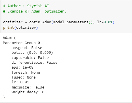
ADAM (Adaptive Moment Estimation)

Adam (Adaptive Moment Estimation), combines ideas from two other popular optimization algorithms RMSProp (Root Mean Square Propagation) and momentum. For more information on please refer Gradient Descent with Momentum section above. It also works on RMSProp mechanism by scaling the learning rate using moving average of squared gradients. Below is the example of Adam: